VIII. Example

This section describes a simple demonstration of the neural network library, using the character classifier which comes with the source code.
This kind of classification is very simple - we are trying to find the best fit, out of a library of known images, to an image corrupted by noise. The noise in this case is modelled in a very simplistic way, that is, in the form of a random number between -MAX and MAX which is added to each sample.
The images are a linear array of floating point numbers which represent the concatenated rows of a 5x7 matrix. If an entry is +1, it is black, if an entry is -1, it is white.

The network contains 35 input nodes (one for each pixel), 60 hidden nodes and 26 output nodes (one for each letter of the English alphabet). When in use (i.e. after training), the network will be loaded with a corrupted image, with a pixel value going to each input node.
At the output, only one node should produce an output close to 1 (actually 0.95) when presented with a given pattern. An alternative scheme would have 7 output nodes to give the binary ascii character which best matches the given input. It may even be possible to adopt a multi-valued logic system, in which you may only need one or two output nodes. It all depends on the training.

Of course, a neural network is not the most efficient nor the most accurate way to solve this particular problem. Simply calculating the covariance between the test image and each reference image, and identifying the best match, is going to be better by any measure of calculation. However, the point of the network is that we don't need to know about covariance - in fact we only need to show it examples of what we want it to do.

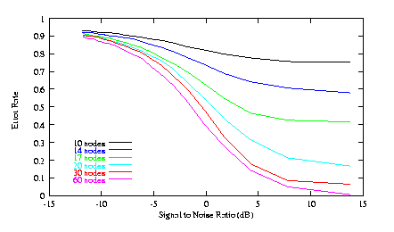
To give you some rough idea of how this network behaves with variations in network parameters, take a look at the following figure:

This shows the performance of the network (measured as an error rate plotted against the signal-to-noise ratio) with differing numbers of hidden-layer nodes. As you can see, more nodes tend to make the network perform better (up to a point).

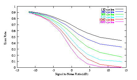
The second graph shows the performance of the network (again as error rate vs. SNR) with a fixed number of hidden-layer nodes, and a number of different levels of training. Again, as you might expect, performance improves (up to a point) with additional training.

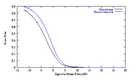
Finally, it is worth comparing the "best" neural network (many hidden layer nodes, and many training cycles) with the optimal statistical technique. As you can see, performance is similar (but worse).
Also, the number of calculations required even in normal operation (ignoring training) is significantly higher. This is the price you must pay for the greater flexibility of a neural network.